
ML from the beginning to the end (For newbies🐢)
Explore and run machine learning code with Kaggle Notebooks | Using data from multiple data sources
www.kaggle.com
[원본 Kaggle kernel] 도움이 되셨다면, Upvote 누르자 >_<
* 해당 포스팅은 간단한 EDA와 Feature engineering을 진행합니다. ML training을 보고 싶다면 다음 포스팅으로!
Fifth. EDA & Visualization -📊
ubiquant = train_set.copy()
1) Check time_id
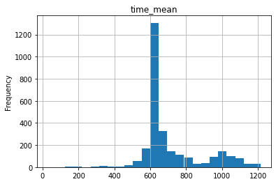
time_id의 분포를 파악하기 위해 time_id를 기준으로 묶었습니다.
각가의 time_id를 가진 investment_id에 count()/ mean() / std() 함수를 써서 그래프로 나타냈습니다.
time_count = ubiquant['time_id'].groupby(ubiquant['investment_id']).count()
time_count.plot(kind='hist', bins=25, grid=True, title='time_count')
plt.show()

time_mean = ubiquant['time_id'].groupby(ubiquant['investment_id']).mean()
time_mean.plot(kind='hist', bins=25, grid=True, title='time_mean')
plt.show()

time_std = ubiquant['time_id'].groupby(ubiquant['investment_id']).std()
time_std.plot(kind='hist', bins=25, grid=True, title='time_std')
plt.show()

del time_count
del time_mean
del time_std


2) Scatter plot
간략하게 Scatter plot로 표현해보았습니다.
from pandas.plotting import scatter_matrix

attri = ['investment_id', 'time_id', 'f_0', 'f_1']
scatter_matrix(ubiquant[attri], figsize = (12,8))

3) Check Outlier
training에 앞서, 이상치를 탐색했습니다.
'investment_id'를 그룹으로 묶은 후, Target의 개수와 평균을 측정했습니다.
investment_count = ubiquant.groupby(['investment_id'])['target'].count()
fig, ax = plt.subplots(1, 1, figsize=(12, 6))
investment_count.plot.hist(bins=60, color = 'blue', alpha = 0.4)
plt.title("Count of investment by target")
plt.show()

investment_mean = ubiquant.groupby(['investment_id'])['target'].mean()
fig, ax = plt.subplots(1, 1, figsize=(12, 6))
investment_mean.plot.hist(bins=60, color = 'blue', alpha = 0.4)
plt.title("Mean of investment by target")
plt.show()

ax = sns.jointplot(x=investment_count, y=investment_mean, kind='reg',
                  height=8, color = 'blue')
ax.ax_joint.set_xlabel('observations')
ax.ax_joint.set_ylabel('mean target')
plt.show()


Sixth. Feature Engineering -🛠
1) Make label
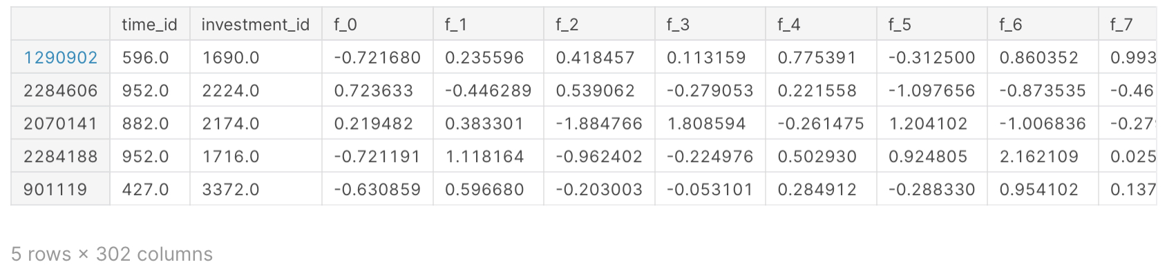
train_x = train_set.drop(['target', 'row_id'], axis=1).copy()
train_target = train_set['target'].copy()
display(train_x.head())
train_target.head()
1290902    1.552734
2284606    8.234375
2070141   -1.006836
2284188   -0.957031
901119     0.775391
Name: target, dtype: float16
2) Remove outlier
그래프에서 나타난 이상치들을 제거합니다.
다만, training을 했을 때 성능이 떨어진다면, 정말 이상치가 맞는 것인지 검사 작업을 해야 합니다.
# Step 2.
outlier_id = investment_mean.reset_index(name='mean')
outlier_id = outlier_id[abs(outlier_id['mean']) < 0.15]
outlier_id = outlier_id['investment_id'].tolist()

# removeing outlier_id
remove_df = train_set[train_set['investment_id'].isin(outlier_id)].copy()
remove_df

이상치를 제거한 후, 그래프를 다시 그려봅니다.
앞서 확인한 그래프에선 이상치 때문에 그래프가 필요없는 부분까지 표현하고 있었습니다. 지금은 본체를 더 크게 표현하고 있습니다. (2,3번째 그래프)
# Step 3.
investment_count = remove_df.groupby(['investment_id'])['target'].count()
fig, ax = plt.subplots(1, 1, figsize=(12, 6))
investment_count.plot.hist(bins=60, color = 'blue', alpha = 0.4)
plt.title("Count of investment by target")
plt.show()

investment_mean = remove_df.groupby(['investment_id'])['target'].mean()
fig, ax = plt.subplots(1, 1, figsize=(12, 6))
investment_mean.plot.hist(bins=60, color = 'blue', alpha = 0.4)
plt.title("Mean of investment by target")
plt.show()

ax = sns.jointplot(x=investment_count, y=investment_mean, kind='reg',
                  height=8, color = 'blue')
ax.ax_joint.set_xlabel('observations')
ax.ax_joint.set_ylabel('mean target')
plt.show()


3) Scaling & Simple pipeline
but f_0 ~ f_300 seem to be similar scale. so we don't need scaling
원래는 각 변수들의 training을 더 원활하게 하기 위해 Scaling을 합니다.
Scaling이란 단위를 비슷하게 만드는 작업을 의미합니다. 하지만 본 대회 데이터는 이미 Scaling이 되어 있는 것으로 보여 코드만 작성하고 실제로 돌리진 않았습니다.
# from sklearn.pipeline import Pipeline
# from sklearn.preprocessing import StandardScaler

# f_num_pipeline = Pipeline([
#     ('std_scaler', StandardScaler())
# ])

# ubi_f_pipe = f_num_pipeline.fit_transform(train_set[features])
del train_set
'👶 Mini Project > Kaggle' 카테고리의 다른 글
| [Kaggle] Ubiquant Market Prediction, 금융데이터 예측 - Part 3 (0) | 2022.04.03 |
|---|---|
| [Kaggle] Ubiquant Market Prediction, 금융데이터 예측 - Part 1 (0) | 2022.04.03 |

